Step 5: Develop your model

When you are developing your model, you want to be able to quickly execute code, see outputs, and make iterative improvements. Domino enables this with Workspaces. Step 3 covered starting a Workspace and explored Workspace options like VSCode, RStudio, and Jupyter.

In this section, we will use Rstudio to load, explore, and transform some data. After the data has been prepared, we will train a model.

Step 5.1: Load and explore the dataset

If you have not done so, complete Step 4 to download the dataset. You should see data.csv in /mnt in files pane. If not, return to Step 4 to download the dataset.
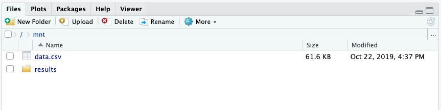
Use the New menu to create a R script and save is as power.R.
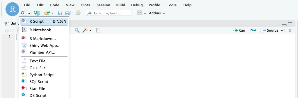
Enter these lines to import some packages:
```
library(tidyverse)
library(lubridate)
```

Create a list of the columns according to information on the column headers at Generation by Fuel Type.

col_names <-  c('HDF', 'date', 'half_hour_increment',
     'CCGT', 'OIL', 'COAL', 'NUCLEAR',
     'WIND', 'PS', 'NPSHYD', 'OCGT',
     'OTHER', 'INTFR', 'INTIRL', 'INTNED',
     'INTEW', 'BIOMASS', 'INTEM')

Read the file you downloaded into a dataframe and set the column names, then display the data:

#Load the data into a data frame
df <- read.csv('data.csv',header = FALSE,col.names = col_names,stringsAsFactors = FALSE)

#remove the first and last row
df <- df[-1,]
df <- df[-nrow(df),]

#Preview the data
View(df)

Execute the script by selecting Code > Source. This opens the content of the df data frame in a new tab:

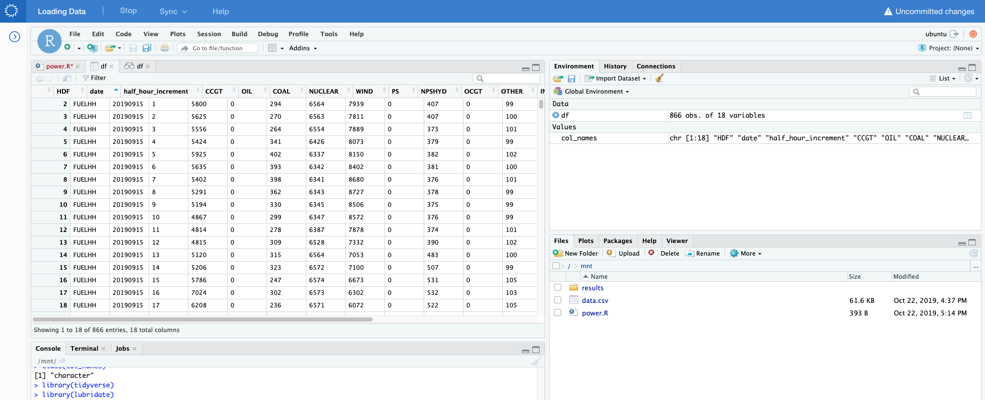
We can see that this is a time series dataset. Each row is a successive half hour increment during the day that details the amount of energy generated by fuel type. Time is specified by the date and half_hour_increment columns.

Tidy that data so that variables are in columns, observations are in rows, and values are in cells. Switch back to the power.R code tab and add the following:

df_tidy <- df %>% gather('CCGT', 'OIL', 'COAL', 'NUCLEAR',
                'WIND', 'PS', 'NPSHYD', 'OCGT',
                'OTHER', 'INTFR', 'INTIRL', 'INTNED',
                'INTEW', 'BIOMASS', 'INTEM', key="fuel", value="megawatt" )

Create a new column datetime that represents the starting datetime of the measured increment. For example, a 20190930 date and 2 half hour increment means that the time period specified is September 19, 2019 from 12:30am to 12:59am.
```
df_tidy <- df_tidy %>% mutate(datetime=as.POSIXct(as.Date(date, "%Y%m%d"))+minutes(30*(half_hour_increment-1)))
```
Visualize the data to see how each fuel type is used during the day by plotting the data.
```
#plot the graph
p <- ggplot(data=df_tidy, aes(x=datetime, y=megawatt, group=fuel)) +
  geom_line(aes(color=fuel))
print(p)
```
Execute the script again by selecting Code > Source. This will update the Plot tab:

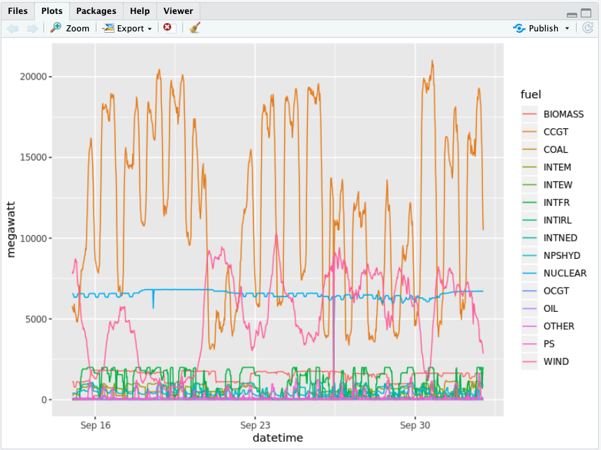
The CCGT column representing "combined-cycle gas turbines" seems to be the most interesting. It generates a lot of energy and is very volatile.

We will concentrate on this column and try to predict the power generation from this fuel source.

Step 5.2: Train a model

Data scientists have access to many libraries and packages that help with model development. Some of the most common for R are randomForest, caret, and nnet. These packages are already installed in the Domino Standard Environment, the default environment. However, there may be times that you want to experiment with a package that is new and not installed in the environment.

We will build a model with the Facebook Prophet package, which is not installed into the default environment. You will see that you can quickly get started with new packages and algorithms just as fast as they are released into the open source community.

In your R console, install Facebook Prophet. This might take >5 minutes to install. If it fails, make sure that you’ve selected a hardware tier with >2gb of ram:

# Install specific version of the prerequisite RcppParallel package as its latest version 5.0.2 fails to install
install.packages('https://cran.r-project.org/src/contrib/Archive/RcppParallel/RcppParallel_5.0.1.tar.gz', repos=NULL, type="source")
# Now install latest version of Facebook Prophet
install.packages('prophet')

For Facebook Prophet, the time series data needs to be in a DataFrame with 2 columns named ds and y. Let’s rename the columns and filter to just to fuel type "CCGT":
```
df_CCGT <- df_tidy %>% filter(fuel=="CCGT") %>% select(datetime,megawatt)

names(df_CCGT) <- c("ds","y")
```

Split the dataset into train and test sets:

split_index <- round(nrow(df_CCGT)*.8)
df_CCGT_train <- df_CCGT[1:split_index,]
df_CCGT_test <- df_CCGT[(split_index+1):nrow(df_CCGT),]

Import Facebook Prophet and fit a model:

library(prophet)
m <- prophet(df_CCGT_train)

Make a DataFrame to hold prediction and predict future values of CCGT power generation:

predict_ln <- round(nrow(df_CCGT_test)/2)
future <- make_future_dataframe(m, periods = predict_ln,freq = 1800 )
forecast <- predict(m, future)

Plot the fitted line with the training and test data:
```
p <- dyplot.prophet(m, forecast)
print(p)
```
Save the code.

Step 5.3: Export the model

Trained models are meant to be used. There is no reason to re-train the model each time you use the model. Export or serialize the model to a file to load and reuse the model later. In R, you can commonly use the saveRDS command to create RDS files.

Export the trained model as an rds file for later use:
```
saveRDS(m, file = "model.rds")
```

We will use the serialized model in Step 7 when we create an API from the model.