Use Snowflake to create a predictive weather model

In this section, you will use Jupyter Notebook to create a predictive model for a single weather station. You will explore the data, create a chart, and finally use the XGBoost library to create the model. This will allow you to predict the weather using the data you have stored in Snowflake.

Note	Each code snippet can fit inside a Juypter Notebook cell. The results displayed are based on data downloaded at the time of writing this tutorial and might not be identical to your results.

Explore the data

Import the necessary libraries and connect to the database:

from domino.data_sources import DataSourceClient
import pandas as pd
import xgboost as xg
import sklearn as sk
from datetime import date, timedelta, datetime
import numpy as np
import os
from pathlib import Path

# Directory in which you will store the model
model_directory = "/mnt/models"

# Hot temperature threshold in degrees Celsius
hot_day_flag = 33

# Instantiate a client and fetch the Data Source instance
ds = DataSourceClient().get_datasource("weather_db")
res = ds.query("select * from state_province")
df = res.to_pandas()
df.head()

Note the following:

The hot_day_flag variable is created to indicate excessively warm days, which will be used in the visualization.
A separate folder is created in which the model will be stored.
The database initialization code allows you to connect to and fetch data from the Snowflake Data Source instance. If the code runs successfully, a list of the states in the database is displayed:
```
    STATE_CODE  NAME
-------------------------------
0   AK          ALASKA
1   AL          ALABAMA
2   AR          ARKANSAS
3   AS          AMERICAN SAMOA
4   AZ          ARIZONA
```

To whittle down your dataset, search for stations that have recorded data from the past 50 years up to the present day. This will help you build a more reliable model; the more data you have, the better its predictive power. You can achieve this by examining the data inventory table:

sfQuery = "SELECT * FROM STATION_DATA_INVENTORY LIMIT 10"
res = ds.query(sfQuery)
df = res.to_pandas()
df.head()

The result:

    ENTRY_ID  STATION_ID    LATITUDE  LONGITUDE  ELEMENT  FIRST_YEAR  LAST_YEAR
----------------------------------------------------------------------------------
0   1044481   AU000005010   48.0500   14.1331    TMIN     1876        2022
1   1044482   AU000005010   48.0500   14.1331    PRCP     1876        2022
2   1044483   AU000005010   48.0500   14.1331    SNWD     1982        2022
3   1044484   AU000005010   48.0500   14.1331    TAVG     1977        2022
4   1044485   AU000005901   48.2331   16.3500    TMAX     1855        2022

Of the features tracked by NOAA, see how many stations tracked them for a fairly good period:

feature_list = ['TMIN','TMAX', 'PRCP', 'RHAV', 'AWND', 'ASTP']

for cur_feature in feature_list:
    sfQuery = f"SELECT COUNT(DISTINCT STATION_ID) AS ELEMENT_COUNT " \
            f"FROM STATION_DATA_INVENTORY WHERE ELEMENT = '{cur_feature}' AND FIRST_YEAR < 1951 AND LAST_YEAR >2021"
    res = ds.query(sfQuery)
    df = res.to_pandas()
    feature_station_count = df.iloc[0,0]
    print(f"The number of stations with 70 years of data for feature {cur_feature} is {feature_station_count}")

The result:

The number of stations with 70 years of data for feature TMIN is 268
The number of stations with 70 years of data for feature TMAX is 265
The number of stations with 70 years of data for feature PRCP is 584
The number of stations with 70 years of data for feature RHAV is 0
The number of stations with 70 years of data for feature AWND is 0
The number of stations with 70 years of data for feature ASTP is 0

It looks like you will need to focus on minimum (TMIN) and maximum (TMAX) temperatures, along with the precipitation (PRCP), as the features for your model. You will rely on the date (i.e. the time of year) to build your predictive model for temperatures.

Find the stations that have all three features for the 70-year period.

Define the query:
```
sfQuery = """SELECT t1.STATION_ID
            FROM
            (SELECT STATION_ID FROM STATION_DATA_INVENTORY WHERE ELEMENT = 'PRCP' AND FIRST_YEAR < 1951 AND LAST_YEAR >2021) t1,
            (SELECT STATION_ID FROM STATION_DATA_INVENTORY WHERE ELEMENT = 'TMIN' AND FIRST_YEAR < 1951 AND LAST_YEAR >2021) t2,
            (SELECT STATION_ID FROM STATION_DATA_INVENTORY WHERE ELEMENT = 'TMAX' AND FIRST_YEAR < 1951 AND LAST_YEAR >2021) t3
            WHERE t1.station_id = t2.STATION_ID AND t1.station_ID = t3.STATION_ID ORDER BY station_id ASC"""
```
In the query, you are asking Snowflake to find the stations that have the features of interest:
- Firstly, it filters the data for all stations that have the PRCP feature by using a subquery. The results from this subquery are stored as t1.
- The second subquery, for which results are stored as t2, filters for stations with the TMIN feature.
- The third subquery, with results stored as t3, contains stations with the TMAX feature.
- The main query filters the results to only include STATION_ID values that are common to results from all three subqueries (by joining the three subqueries on STATION_ID).

Next, run the query:

res = ds.query(sfQuery)
df_station_with_data = res.to_pandas()
df_station_with_data.head()

The query result:

    STATION_ID
----------------
0   AU000005901
1   AU000006306
2   AU000011801
3   AU000016402
4   BE000006447

Use the first station on the list:
```
station_to_check = 'AU000005901'
```

Find where this station is located:

sfQuery = f"""SELECT *
            FROM WEATHER_STATION WS, COUNTRY C
            WHERE WS.STATION_ID = '{station_to_check}'
            AND C.COUNTRY_ID = SUBSTRING ('{station_to_check}', 1, 2)"""

res = ds.query(sfQuery)
station_data_df = res.to_pandas()
station_data_df.head()

You will see the following:

    STATION_ID   LATITUDE  LONGITUDE  ELEVATION  STATION_STATE  STATION_NAME  GSN  HCN_CRN  WMO_ID  COUNTRY_ID  COUNTRY_NAME
-----------------------------------------------------------------------------------------------------------------------------
0   AU000005901  48.2331   16.35      199.0                     WIEN          GSN           11035   AU          Austria

You are joining two tables: WEATHER_STATION and COUNTRY. The COUNTRY table uses two characters for its COUNTRY_ID field, which are the first two characters in the STATION_ID. You can therefore join the two tables on that field to get the full country name - Austria in this case.

Have a look at the first few lines of this data:

sfQuery = f"""SELECT *
            FROM STATION_DATA_INVENTORY
            WHERE STATION_ID = '{station_to_check}'"""

res = ds.query(sfQuery)
df = res.to_pandas()
df.head()

The output:

    ENTRY_ID  STATION_ID    LATITUDE  LONGITUDE  ELEMENT  FIRST_YEAR  LAST_YEAR
----------------------------------------------------------------------------------
0   1044485   AU000005901   48.2331   16.35      TMAX     1855        2022
1   1044486   AU000005901   48.2331   16.35      TMIN     1855        2022
2   1044487   AU000005901   48.2331   16.35      PRCP     1901        2022
3   1044488   AU000005901   48.2331   16.35      SNWD     1916        2022
4   1044489   AU000005901   48.2331   16.35      TAVG     1952        2022

The results confirm that the features you need are indeed provided by the stations in the list within the station_to_check_df dataframe.

Determine how many stations match this criteria:
```
len(df_station_with_data)
```
This result is:
```
250
```
Therefore, there are 250 stations in the dataset you can use to build a model.

Finally, dive into the actual weather data in the STATION_DATA table. Find how much data the 250 stations have that meet your criteria.

Define the query:

sfQuery = """SELECT COUNT(*)
            FROM STATION_DATA
            WHERE STATION_ID IN
            (SELECT t1.STATION_ID
                FROM
                    (SELECT STATION_ID FROM STATION_DATA_INVENTORY WHERE ELEMENT = 'PRCP' AND
                    FIRST_YEAR < 1951 AND LAST_YEAR >2021) t1,
                    (SELECT STATION_ID FROM STATION_DATA_INVENTORY WHERE ELEMENT = 'TMIN' AND
                    FIRST_YEAR < 1951 AND LAST_YEAR >2021) t2,
                    (SELECT STATION_ID FROM STATION_DATA_INVENTORY WHERE ELEMENT = 'TMAX' AND
                    FIRST_YEAR < 1951 AND LAST_YEAR >2021) t3
                WHERE t1.station_id = t2.STATION_ID AND t1.station_ID = t3.STATION_ID)
            AND DATA_DATE > to_date('1949-12-31')
            ORDER BY STATION_ID ASC, DATA_DATE ASC"""

This query uses the previous query (stations that have the features from 1950 onward) as a subquery and only loads the data since the first day of 1950. It orders the data by station ID and the dates of each reading.

Run the query:
```
res = ds.query(sfQuery)
data_df = res.to_pandas()
data_df
```
This will return:
```
    COUNT(*)
-------------
0   27003504
```
The result shows that there are about 27 million data rows related to your stations alone (this number may differ in your results as NOAA adds new data over time). That’s a pretty big number to hold in memory in a dataframe!

You don’t really need all that data in memory to develop your model. You can start with one station instead. Look at the station data table using a station that you chose at random:

sfQuery = f"""SELECT *
            FROM STATION_DATA
            WHERE STATION_ID = '{station_to_check}'
            AND DATA_DATE > to_date('1949-12-31')
            ORDER BY DATA_DATE ASC
            LIMIT 10"""

res = ds.query(sfQuery)
df = res.to_pandas()
df

The table result:

    ENTRY_ID  STATION_ID   ELEMENT  ELEMENT_VALUE
-------------------------------------------------
0   755       AU000005901  SNWD       0
1   752       AU000005901  TMAX     -11
2   753       AU000005901  TMIN     -49
3   754       AU000005901  PRCP       0
4   323815    AU000005901  PRCP      85
5   323813    AU000005901  TMAX      46
6   323814    AU000005901  TMIN     -76
7   323816    AU000005901  SNWD       0
8   648137    AU000005901  SNWD       0
9   648136    AU000005901  PRCP       4

From the STATION_DATA table, we only need the following features:

ENTRY_ID - The sequential unique ID for the data item (on the date the data was captured).
STATION_ID - The weather station’s unique identifier.
DATA_DATE - The date on which the data was captured.
ELEMENT - The data that was measured (precipitation or temperature).
ELEMENT_VALUE - The measurement value.

Note that there are multiple rows of data per day for this station. It will be easier to train your regression model if you associate the data with each day instead. That way, each row will have the date, precipitation, and temperatures as features, instead of one feature per row.

Wrangle the data

Run a single query to obtain all the data, and then reshape it into a new, date-based dataframe. Start by getting the data you need for the station:

# Get all data for the current station
sfQuery = f"""SELECT DATA_DATE, ELEMENT, ELEMENT_VALUE
            FROM STATION_DATA
            WHERE STATION_ID = '{station_to_check}'
            AND DATA_DATE > to_date('1949-12-31')
            AND (ELEMENT = 'PRCP' OR ELEMENT = 'TMIN' OR ELEMENT = 'TMAX')
            ORDER BY DATA_DATE ASC"""

res = ds.query(sfQuery)
station_data_full = res.to_pandas()
station_data_full.size

The result:

Therefore, there are almost 85 000 records with multiple readings per day. (Note that this number may differ in your results as NOAA adds new data over time.)

Remove duplicates from the data, if any exist, and see how many rows are left:

dupes = station_data_full[station_data_full.duplicated()]

if len(dupes) > 0:
    station_data_full = station_data_full.drop_duplicates()

# See how many rows are left after we remove the duplicates
print(len(station_data_full))

The result:

We removed close to 3 000 duplicates from the data.

Now check for missing data:

# Date of last record in the dataframe
latest_date = station_data_full.iloc[-1]['DATA_DATE']

# See where the data is missing
station_data_full = station_data_full.set_index('DATA_DATE')
missing_dates = pd.date_range(start='1950-1-1', end=latest_date).difference(station_data_full.index)
print(missing_dates)

The result:

DatetimeIndex(['2022-04-19', '2022-12-15', '2024-05-01'], dtype='datetime64[ns]', freq=None)

(This may differ from your results as NOAA adds new data over time.)

Looking at the data, how many dates are missing per year?
```
len(missing_dates)
```
Based on the output, 3 dates are missing some data.

Iterate over this date list and add three new rows for each date that is missing - one for each feature (TMIN, TMAX, and PRCP).

# Add missing dates to the dataframe
element_list = ['PRCP', 'TMIN', 'TMAX']

for missing_date in missing_dates:
    cur_date = pd.to_datetime(missing_date).date()
    for cur_element in element_list:
        missing_row_test=station_data_full[(station_data_full['DATA_DATE'] == cur_date) & (station_data_full['ELEMENT'] == cur_element)]
        if len(missing_row_test) == 0:
            new_row = pd.DataFrame({'DATA_DATE': cur_date, 'ELEMENT': cur_element, 'ELEMENT_VALUE': np.NaN}, index=['DATA_DATE'])
            station_data_full = pd.concat([station_data_full, new_row], ignore_index=True)

Check how well you did with one of the missing dates:

rows_for_date = station_data_full[station_data_full['DATA_DATE'] == date(2024, 5,1)]
print(rows_for_date)

The result:

        DATA_DATE   ELEMENT  ELEMENT_VALUE
------------------------------------------
81332   2024-05-01  PRCP     NaN
81333   2024-05-01  TMIN     NaN
81334   2024-05-01  TMAX     NaN

The dates that were missing are now included in the dataframe.

Next, create a new dataframe that will be date-oriented, where each row will consist of a DATA_DATE, TMAX value, TMIN value, and PRCP value.

Create and populate individual dataframes for each feature, starting with TMAX:

tmax_df = station_data_full[station_data_full['ELEMENT'] == 'TMAX']
tmax_df = tmax_df[["DATA_DATE", "ELEMENT_VALUE"]]
tmax_df = tmax_df.rename(columns={"ELEMENT_VALUE": "TMAX"})
tmax_df.head()

The result:

    DATA_DATE   TMAX
----------------------
2   1950-01-01  -11.0
4   1950-01-02   46.0
8   1950-01-03   46.0
11  1950-01-04   37.0
14  1950-01-05    4.0

Then for TMIN:

tmin_df = station_data_full[station_data_full['ELEMENT'] == 'TMIN']
tmin_df = tmin_df[["DATA_DATE", "ELEMENT_VALUE"]]
tmin_df = tmin_df.rename(columns={"ELEMENT_VALUE": "TMIN"})

Then for PRCP:

prcp_df = station_data_full[station_data_full['ELEMENT'] == 'PRCP']
prcp_df = prcp_df[["DATA_DATE", "ELEMENT_VALUE"]]
prcp_df = prcp_df.rename(columns={"ELEMENT_VALUE": "PRCP"})

Join all three dataframes on the date:

station_data_merged = tmax_df.merge(tmin_df, on="DATA_DATE", how="left")
station_data_merged = station_data_merged.merge(prcp_df, on="DATA_DATE", how="left")
station_data_merged.head()

This will create a dataframe that looks something like this:

    DATA_DATE   TMAX  TMIN   PRCP
----------------------------------
0  1950-01-01  -11.0  -49.0   0.0
1  1950-01-02   46.0  -76.0  85.0
2  1950-01-03   46.0   17.0   4.0
3  1950-01-04   37.0    3.0   3.0
4  1950-01-05    4.0  -18.0  63.0

If you look at the number of rows in this merged dataframe, you will see that the results correspond to 70+ years of data:
```
len(station_data_merged) / 365
```
The result:
```
75.11780821917809
```

NOAA saves temperature data in tenths of degrees. Therefore, you need to divide the temperature columns by 10.

station_data_merged['TMAX'] = station_data_merged['TMAX']/10;
station_data_merged['TMIN'] = station_data_merged['TMIN']/10;
station_data_merged.head()

The dataframe now looks like this:

    DATA_DATE  TMAX  TMIN  PRCP
--------------------------------
0  1950-01-01  -1.1  -4.9   0.0
1  1950-01-02   4.6  -7.6  85.0
2  1950-01-03   4.6   1.7   4.0
3  1950-01-04   3.7   0.3   3.0
4  1950-01-05   0.4  -1.8  63.0

Impute the data

Use the interpolate() method from Pandas to fill the missing dates.

First, ensure that the dataframe is ordered by date and that no duplicate rows exist:
```
station_data_merged = station_data_merged.sort_values(by=['DATA_DATE'])
station_data_merged = station_data_merged.drop_duplicates()
station_data_merged['DATA_DATE'] = pd.to_datetime(station_data_merged['DATA_DATE'])
```
Note that in the last statement, you converted the DATA_DATE column to be of type datetime. That is important because you are going to interpolate data that is part of a time series, and Pandas requires the date to be the index in order to enable time-based interpolation.

Convert the index to the date column:

station_data_merged = station_data_merged.set_index('DATA_DATE')

Finally, interpolate the missing dates in the series:

station_data_merged['TMAX'] = station_data_merged['TMAX'].interpolate(method='time', limit_direction='backward')
station_data_merged['TMIN'] = station_data_merged['TMIN'].interpolate(method='time', limit_direction='backward')
station_data_merged['PRCP'] = station_data_merged['PRCP'].interpolate(method='time', limit_direction='backward')

Check on one of the dates that was previously missing:
```
station_data_merged.loc['2024-05-01']
```
The above command returns the following result:
```
TMAX    2.370000
TMIN    1.240000
PRCP    6.666667
Name: 2024-05-01 00:00:00, dtype: float64
```
The missing values were filled through the interpolation.

Make sense of the data

How many days can be regarded as hot weather days? A good number to use is 90° Fahrenheit (33° Celsius). Find how many days per year were considered hot days.

Start by flagging days as hot if they exceeded a temperature of 33° Celsius:

hot_day_df = station_data_merged.copy()
hot_day_df['hot_day'] = hot_day_df['TMAX'] > hot_day_flag
hot_day_df.head()

The flag is now added to the dataframe:

DATA_DATE   TMAX  TMIN  PRCP  hot_day
--------------------------------------
1950-01-01  -1.1  -4.9   0.0  False
1950-01-02   4.6  -7.6  85.0  False
1950-01-03   4.6   1.7   4.0  False
1950-01-04   3.7   0.3   3.0  False
1950-01-05   0.4  -1.8  63.0  False

How many hot days were experienced during these 70 years?
```
len(hot_day_df[hot_day_df['hot_day'] == True])
```
It looks like this station had 231 hot days. (Note that this number may differ as NOAA adds new data over time.)

Find out how many hot days there were every year:

hot_day_df['DATA_DATE'] = pd.to_datetime(hot_day_df.index.date)

# Separate the year into its own dataframe column
hot_day_df['year'] = pd.DatetimeIndex(hot_day_df['DATA_DATE']).year
hot_day_summary = hot_day_df.groupby('year')['hot_day'].apply(lambda x: (x==True).sum()).reset_index(name='count')

# Show the top 10 years with the most hot days
hot_day_summary.head(10)

Here, you extract the year, from the index into its own dataframe column, and then apply a lambda function to count how many hot days were experienced in each year.

    year   count
----------------
0   1950   3
1   1951   0
2   1952   2
3   1953   0
4   1954   0
5   1955   0
6   1956   0
7   1957   7
8   1958   0
9   1959   0

Now determine the hottest temperature in each year:

hottest_temp_in_year = hot_day_df.groupby('year')['TMAX'].max()
hottest_temp_in_year.head(10)

This returns the following output:

year
1950    32.0
1951    32.0
1952    35.7
1953    31.9
1954    32.1
1955    31.5
1956    28.8
1957    35.5
1958    29.6
1959    36.2
Name: TMAX, dtype: float64

Visualize the data

Merge the two dataframes you just created so that you can visualize the data:

hot_day_summary = pd.merge(hot_day_summary, hottest_temp_in_year, on="year")

# Sort data based on the number of hot days in each year
sorted_hot_day_summary = hot_day_summary.sort_values(by = ['count'], ascending=False)
sorted_hot_day_summary.head(10)

The result:

     year   count   TMAX
-------------------------
65   2015   25      37.1
67   2017   13      38.4
72   2022   12      36.3
53   2003   12      37.6
42   1992   12      36.4
63   2013   11      38.5
69   2019   11      37.0
62   2012   10      36.3
68   2018    9      35.2
73   2023    8      36.2

Now visualize the data in a histogram. You may notice extreme deviations in years where too much data is missing and it could not be interpolated properly.

ax = hot_day_summary.plot(y=['TMAX'], kind='line', color='red', marker='*', figsize=(15,15))
ax2 = hot_day_summary.plot(y=['count'], ax=ax, kind='bar', color='blue', secondary_y=True)
ax.set_xticks(hot_day_summary.index, hot_day_summary.year)
ax.set_xlabel('Year')
ax.set_ylabel('Hottest Day Temperature')
ax2.set_ylabel('Number of Hot Days')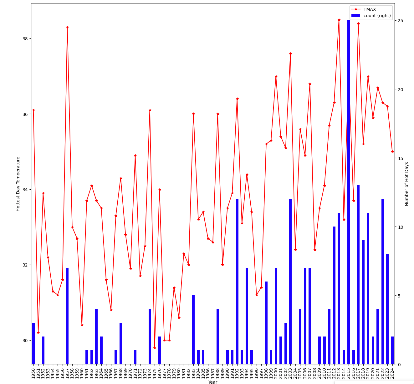

Create a predictive model

Now that you have the data you need for a single station, you can create a predictive model by using the XGBoost library and build the model using linear regression.

The parts of each date are features you’ll use for your model. Therefore, first split the date, which is currently the index of the dataframe, into individual columns:

station_data_merged['day'] = station_data_merged.index.day
station_data_merged['month'] = station_data_merged.index.month
station_data_merged['year'] = station_data_merged.index.year
station_data_merged.head()

The output:

DATA_DATE   TMAX  TMIN  PRCP  day  month  year
-----------------------------------------------
1950-01-01  -1.1  -4.9   0.0   1    1     1950
1950-01-02   4.6  -7.6  85.0   2    1     1950
1950-01-03   4.6   1.7   4.0   3    1     1950
1950-01-04   3.7   0.3   3.0   4    1     1950
1950-01-05   0.4  -1.8  63.0   5    1     1950

Create the following two dataframes:
- One dataframe containing the predictive features.
- One dataframe containing the target values (TMAX) that you want to predict.
  X = station_data_merged[['TMIN', 'PRCP', 'day', 'month', 'year']] Y = station_data_merged['TMAX']

Split the dataframes into training and testing dataframes using Scikit-Learn’s train_test_split method.

X_train, X_test, Y_train, Y_test = sk.model_selection.train_test_split(X, Y, test_size = 0.3, random_state = 101)

Now you can go ahead and use XGBoost’s regression capability to create the predictive model:

regressor = xg.XGBRegressor(max_depth=5, learning_rate = 0.3, n_estimators=100, subsample = 0.75, booster='gbtree')
tmax_model = regressor.fit(X_train, Y_train)
prediction = tmax_model.predict(X_test)

To see how well your model predicts:

Calculate the mean squared error:

mse = sk.metrics.mean_squared_error(Y_test, prediction)
print("MSE: %.2f" % mse)

The output:

MSE: 9.53

The output:

Coefficient of determination: 0.85

Predict tomorrow’s weather for this location

To predict tomorrow’s maximum temperature for this location, you will need to do the following:

Create a dataframe to submit to the prediction algorithm.
Get tomorrow’s date and insert it into the day, month, and year columns.
Get the median TMIN and PRCP from all days with the same date in your data sample and set those values for TMIN and PRCP in the dataframe.
Run the prediction and get the predicted maximum temperature.

Here are the steps to achieve the above:

List the inputs that your predictive model requires:
```
X_test.dtypes
```
The result:
```
TMIN     float64
PRCP     float64
day        int64
month      int64
year       int64
dtype: object
```
In other words, the model requires a dataframe with date components (day, month, year), minimum temperature (TMIN), and precipitation (PRCP) as inputs.

Create a dataframe for tomorrow, maintaining column names and data types. (Note that your current date and weather station will affect what the data will look like.)

tomorrow_df = pd.DataFrame({'TMIN': pd.Series(dtype='float64'),
                            'PRCP': pd.Series(dtype='float64'),
                            'day': pd.Series(dtype='int'),
                            'month': pd.Series(dtype='int'),
                            'year': pd.Series(dtype='int')})
tomorrow_date = datetime.now() + timedelta(1)
tomorrow_df.loc[0, 'day'] = tomorrow_date.day
tomorrow_df.loc[0, 'month'] = tomorrow_date.month
tomorrow_df.loc[0, 'year'] = tomorrow_date.year
tomorrow_df

Which will return:

   TMIN  PRCP  day   month  year
-----------------------------------
0  NaN   NaN   18.0  7.0    2024.0

To figure out what values to use for TMIN and PRCP for tomorrow, find the median value across history for tomorrow’s date (in this case, for January 23).

tomorrow_historical = station_data_merged[(station_data_merged['day'] == tomorrow_date.day) & (station_data_merged['month'] == tomorrow_date.month)]
tomorrow_historical

The result:

DATA_DATE   TMAX  TMIN  PRCP  day  month  year
------------------------------------------------
1950-07-18  26.5  16.8   0.0   18    7     1950
1951-07-18  24.1  16.0   0.0   18    7     1951
1952-07-18  26.3  14.6   0.0   18    7     1952
1953-07-18  32.2  17.9   9.0   18    7     1953
1954-07-18  23.0  15.9  34.0   18    7     1954
...         ...   ...   ...    ...   ...   ...
2019-07-18  26.7  16.1   2.0   18    7     2019
2020-07-18  20.0  13.2  93.0   18    7     2020
2021-07-18  26.7  18.0  40.0   18    7     2021
2022-07-18  29.7  13.3  40.5   18    7     2022
2023-07-18  31.4  22.6   0.0   18    7     2023

74 rows x 6 columns

Calculate the median TMIN and PRCP for tomorrow’s date:

tomorrow_df.loc[0, 'TMIN'] = tomorrow_historical['TMIN'].median()
tomorrow_df.loc[0, 'PRCP'] = tomorrow_historical['PRCP'].median()
tomorrow_df

The result:

   TMIN  PRCP  day   month  year
-----------------------------------
0  16.0   0.0  18.0  7.0    2024.0

Now you can go ahead and run your prediction, then format the results to look human readable:

# Use the dataframe in the predict function
prediction = tmax_model.predict(tomorrow_df)

# Format the result
date_str = tomorrow_date.strftime("%A, %B %-d, %Y")
country_name = station_data_df.loc[0, 'COUNTRY_NAME'].strip()
station_name = station_data_df.loc[0, 'STATION_NAME'].strip()

result_output = f"The predicted weather for {station_name}"
result_output = result_output + f", {country_name} for tomorrow, {date_str}, is: {round(prediction[0],0)}\xb0c"
print(result_output)

The result for this location and date is:

The predicted weather for WIEN, Austria for tomorrow, Thursday, July 18, 2024, is: 29.0°

Since you now have a trained model, you can save it for future use and avoid having to repeat the work you just did:

# Check if the output directory exists
if not os.path.exists(model_directory):
    os.mkdir(model_directory)

model_file_path = f"{model_directory}/{station_to_check}.json"
tmax_model.save_model(model_file_path)

You should now see a predictive model file for the location you picked in your JupyterLab session directory.

Next steps

Convert the predictive model you created into a Domino-hosted Domino endpoint.