Deploy your Python model

After you have developed your model and deemed it good enough to be useful, you will want to deploy it. There is no single deployment method that is best for all models. Therefore, Domino offers four different deployment options. One may fit your needs better than the others depending on your use case.

The available deployment methods are:

Scheduled reports
Launchers
Web applications
Model APIs

The remaining sections of this tutorial are not dependent on each other. For example, you will not need to complete the Scheduled report section to understand and complete the Web application section.

Package setup

A prerequisite to the following sections is to install a few packages. To do this, you create a requirements.txt file in the project, which installs the Python packages listed in the file prior to every job or workspace session.

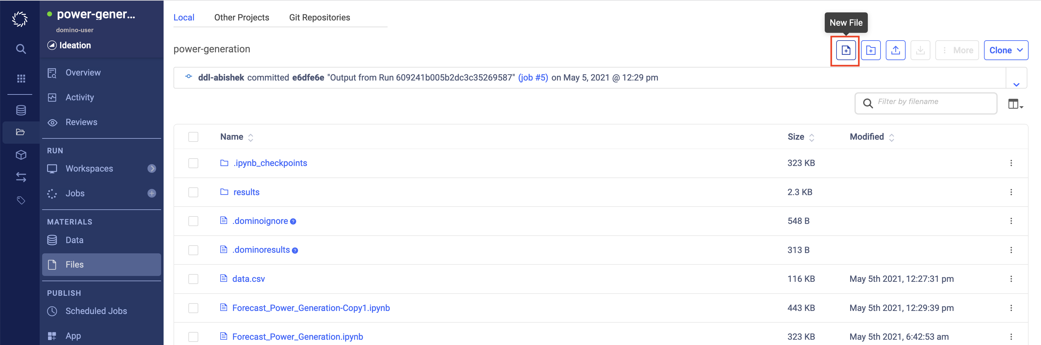
Go to the Files page of your project.
Click New File.

Name it requirements.txt, copy and paste the following contents, and Save:

convertdate
pyqt5<5.12
jupyter-client>6.0.0
nbformat>5.0
papermill<2.0.0
pystan==2.17.1.0
plotly<4.0.0
dash
requests
nbconvert >= 5.4

If you want to install these libraries permanently into a custom environment, find out more in the Model API tutorial.

Scheduled reports

The Scheduled Jobs feature in Domino allows you to run a script on a regular basis. In Domino, you can also schedule a notebook to run from top to bottom and export the resulting notebook as an HTML file. Since notebooks can be formatted with plain text and embedded graphics, you can use the scheduling feature to create regularly scheduled, automated reports for your stakeholders.

In our case, we can imagine that each day we receive new data on power usage. To make sure our predictions are as accurate as possible, we can schedule our notebook to re-train our model with the latest data and update the visualization accordingly.

Start a new Jupyter session.
Select the Jupyter notebook you created when you developed your Python model.
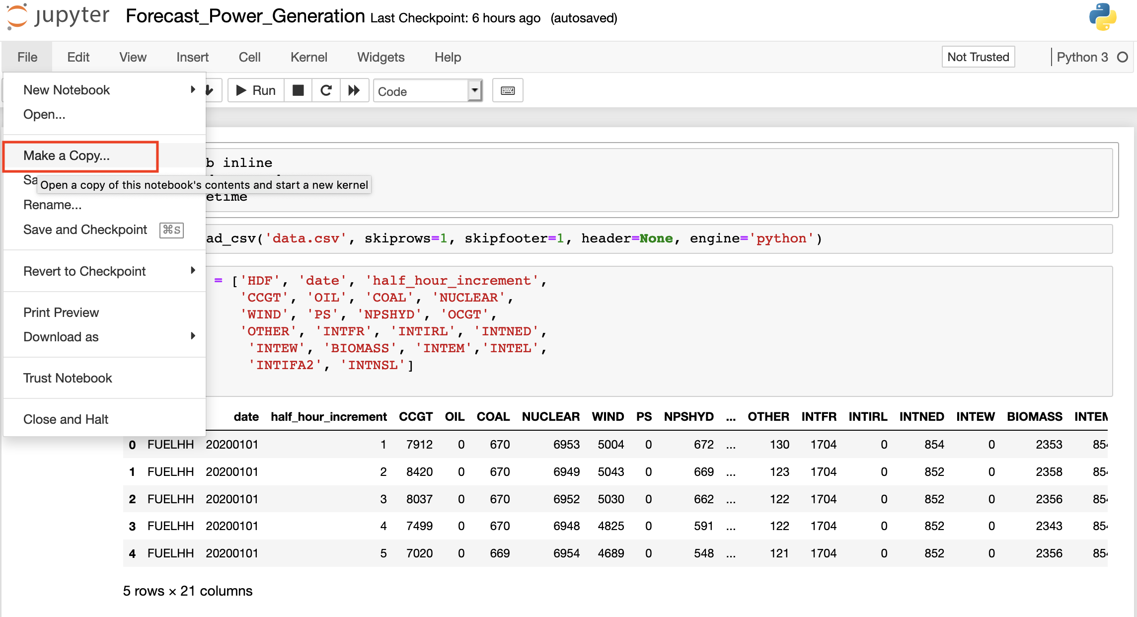
Go to File > Make a copy to create a copy of the notebook.

Add some dynamically generated text to the upcoming report. We want to pull the last 30 days of data.

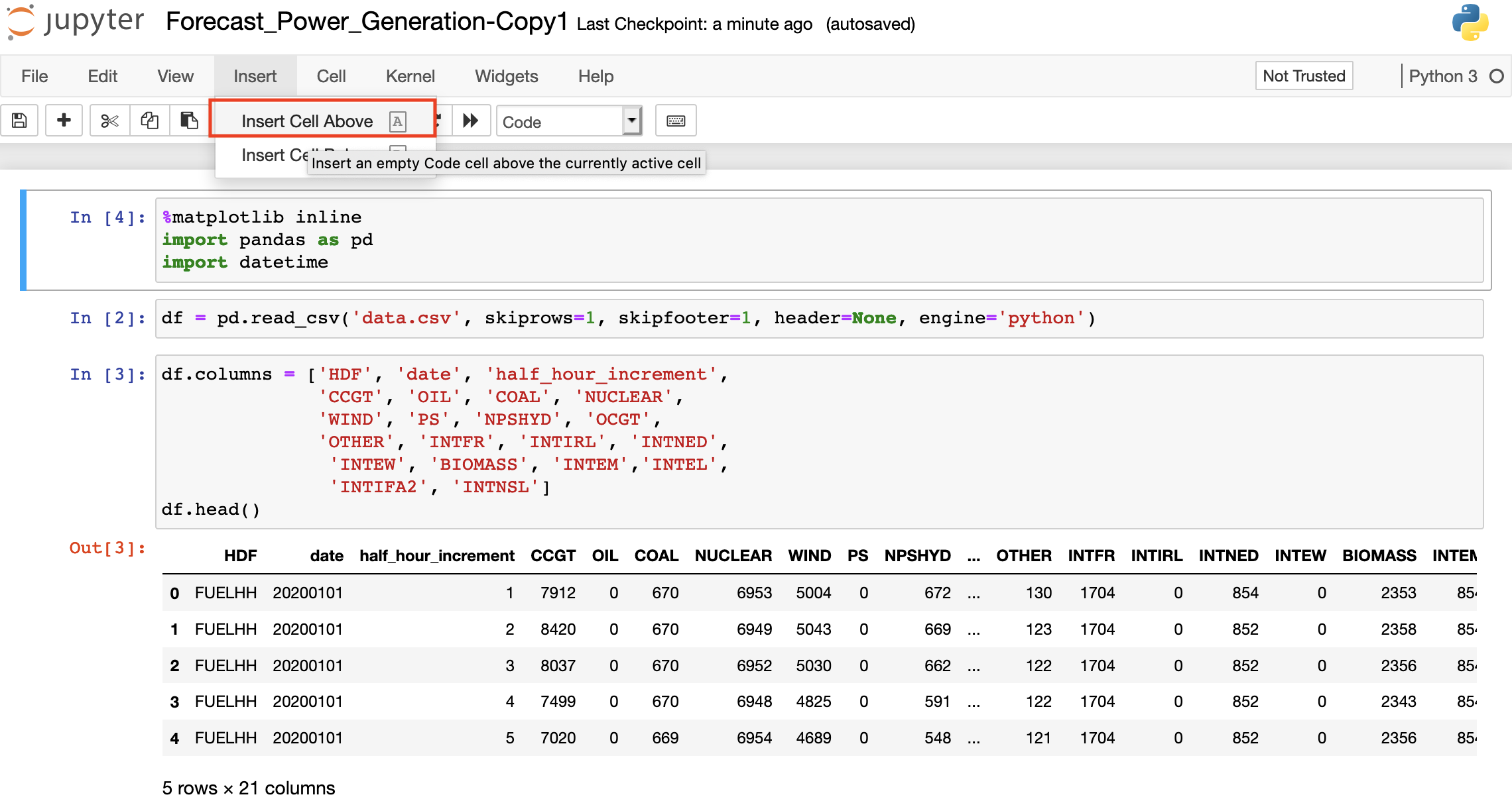
Insert a new cell before the first cell by selecting the first cell and selecting Insert Cell Above.

Copy and paste the following code into the new cell:

import datetime
today = datetime.datetime.today().strftime('%Y-%m-%d')
one_month = (datetime.datetime.today() - datetime.timedelta(30)).strftime('%Y-%m-%d')
!curl -o data.csv "https://www.bmreports.com/bmrs/?q=ajax/filter_csv_download/FUELHH/csv/FromDate%3D{one_month}%26ToDate%3D{today}/&filename=GenerationbyFuelType_20191002_1657" 2>/dev/null

Since this is a report, you will want to add some commentary to guide the reader. For this exercise, we will just add a header to the report at the top. To add a Markdown cell:
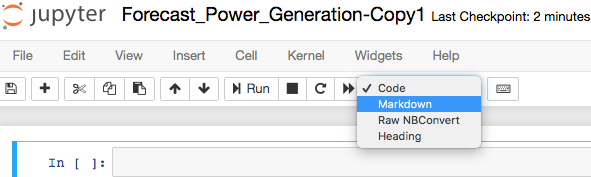
1. Insert a new cell before the first cell again by selecting the first cell and selecting Insert Cell Above.
2. Change the cell type to Markdown.
3. Enter the following in the new Markdown cell:
  # New Predictions for Combined Cycle Gas Turbine Generations
Save the notebook.
Sync All Changes in the workspace session.
Test the notebook.
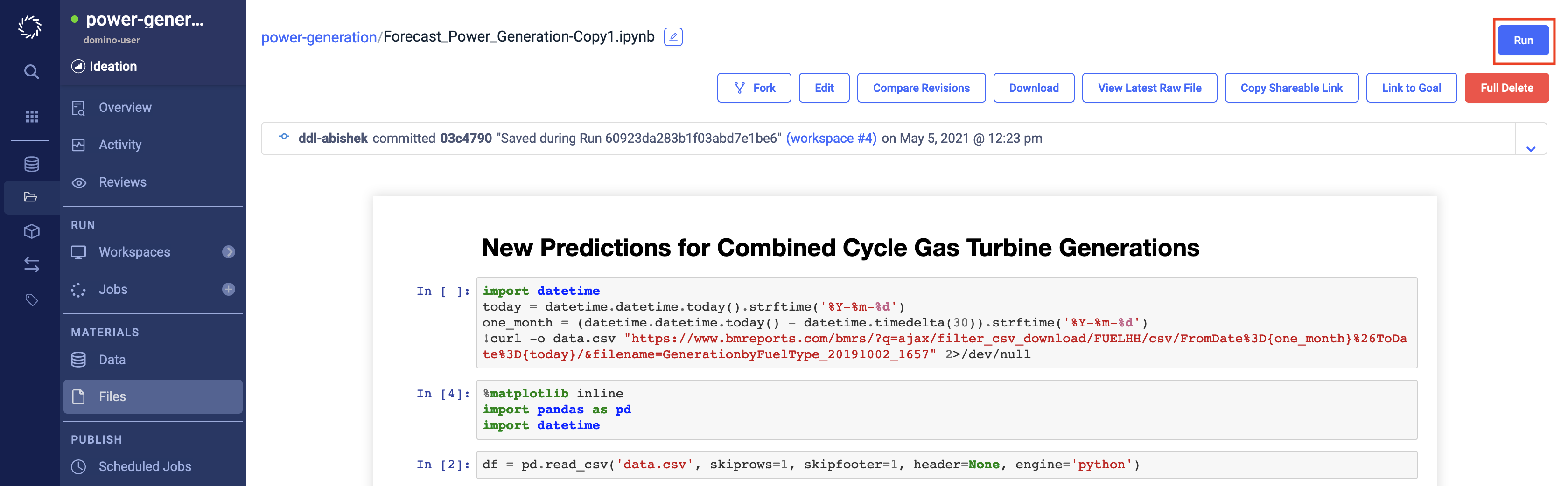
1. Go the Files page.
2. Click the link for the new copy of the notebook.
3. Click Run.
4. Click Start on the modal.
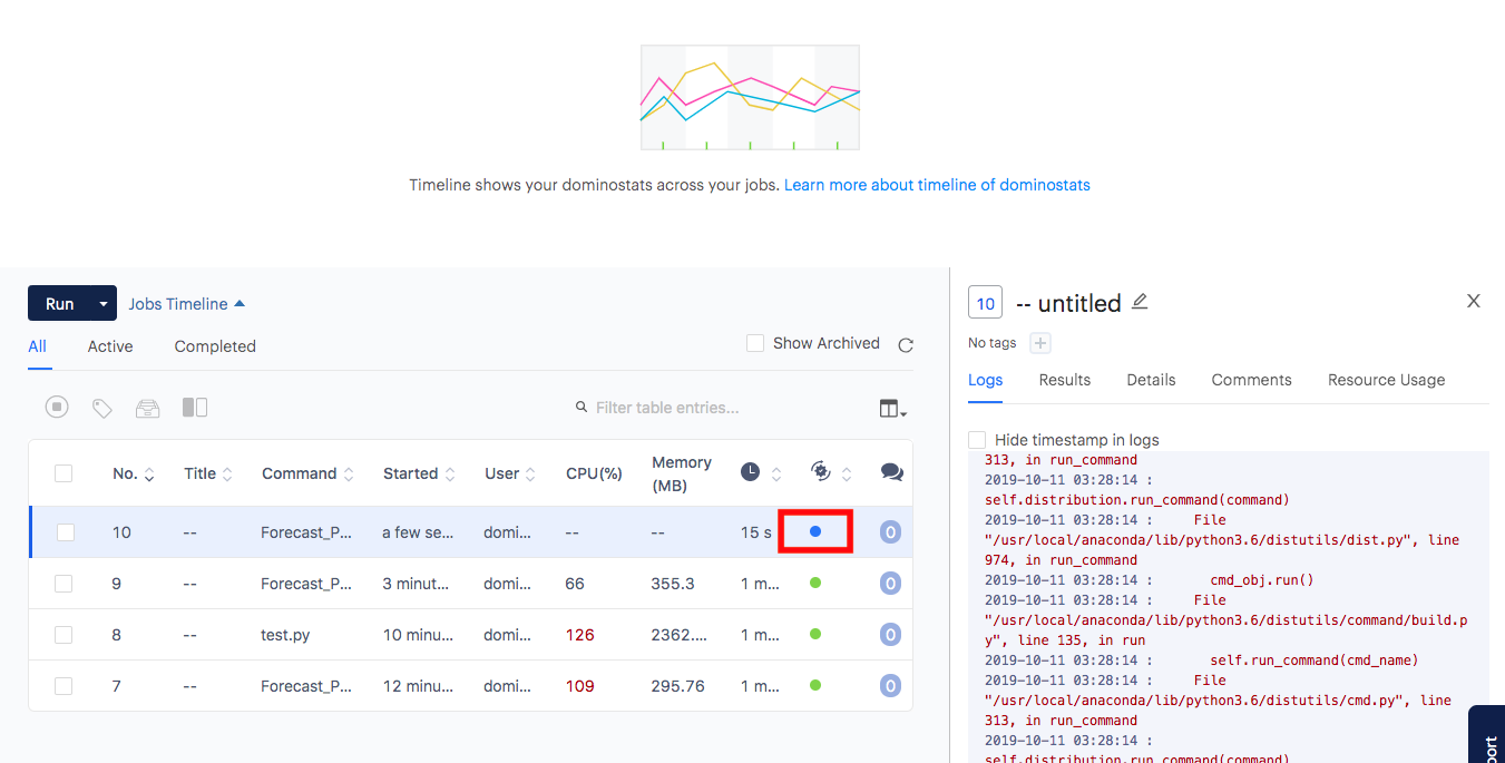
5. Wait for the run to complete. While running, the Status icon will appear blue. Click a job to view its logs.
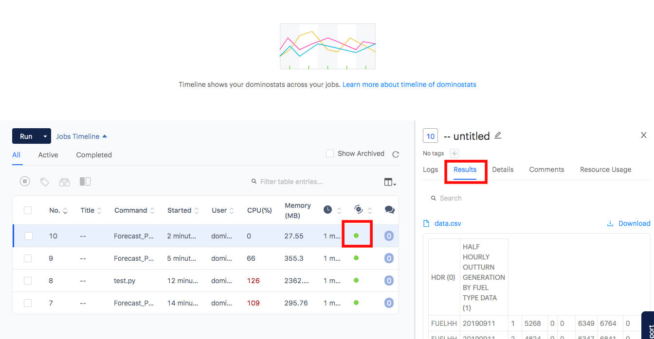
6. After the job has completed successfully, you’ll see the Status icon turn green. You can then browse the Results tab.
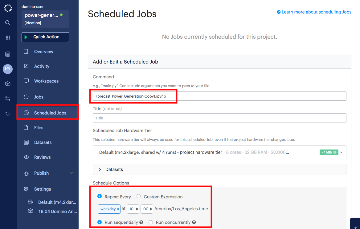
At this point, you can schedule the notebook to run every day. Go to the Scheduled Jobs page.
Start a new scheduled job and enter the name of the file that you want to schedule to run. This will be the name of your Jupyter notebook.
Select how often and when to run the file.
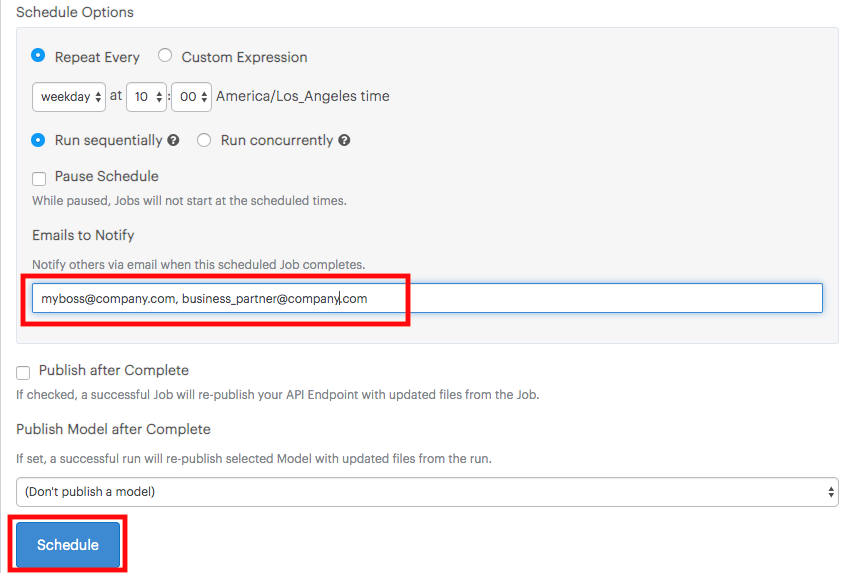
Enter emails of people to send the resulting file(s) to.
Click Schedule.

To learn how to customize the resulting email, see Set Custom Execution Notifications.

Launchers

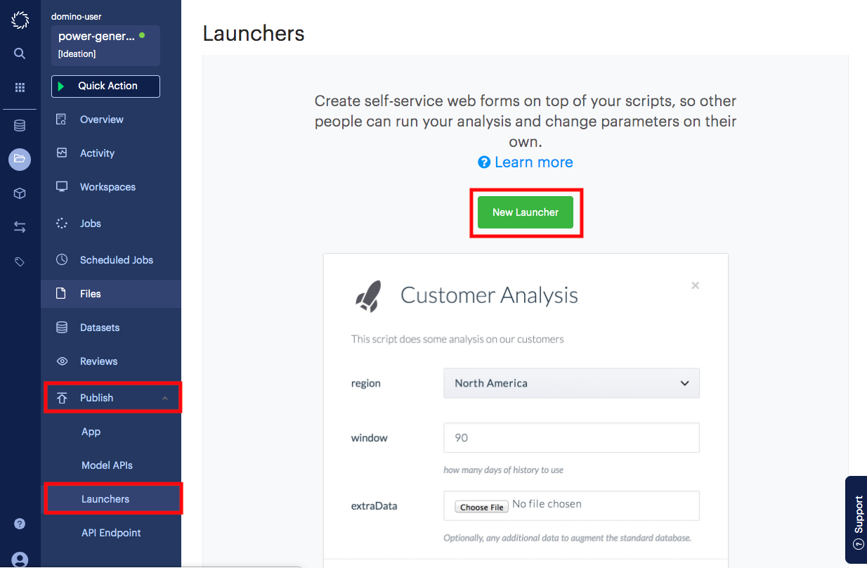
Launchers are web forms that allow users to run templatized scripts. They are especially useful if your script has command line arguments that dynamically change the way the script executes. For heavily customized scripts, those command line arguments can quickly get complicated. Launcher allows you to expose all of that as a simple web form.

Typically, we parameterize script files (i.e. files that end in .py, .R, or .sh). Since we have been working with Jupyter notebooks until now, we will parameterize a copy of the Jupyter notebook that we created when we developed the Python model.

To do so, we will insert a few new lines of code into a copy of the Jupyter notebook, create a wrapper file to execute, and configure a Launcher.

Parameterize the notebook with a Papermill tag and a few edits:
1. Start a Jupyter session. Make sure you are using a Jupyter workspace, not a Jupyterlab workspace. We recently added the requirements.txt file, so the session will take longer to start.
2. Create a copy of the notebook that you created when you developed your Python model. Rename it to Forecast_Power_Generation_for_Launcher.
3. In the Jupyter menu bar, select View/Cell Toolbar/Tags.
4. Create a new cell at the top of the notebook and enter the following into the cell:
  !pip install fbprophet==0.6
5. Create another new cell.
6. Add a parameters tag to the top cell.
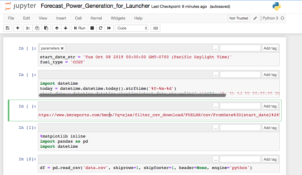
7. Enter the following into the cell to create default parameters:
  start_date_str = 'Tue Oct 06 2020 00:00:00 GMT-0700 (Pacific Daylight Time)' fuel_type = 'CCGT'
8. Insert another cell.
9. Launcher parameters get passed to the notebook as strings. The notebook will need the date parameters to be in a differently formatted string.
  import datetime today = datetime.datetime.today().strftime('%Y-%m-%d') start_date = datetime.datetime.strptime(start_date_str.split(' (')[0], '%a %b %d %Y 00:00:00 GMT%z').strftime('%Y-%m-%d')
10. Insert another new cell with the following code:
  !curl -o data.csv "https://www.bmreports.com/bmrs/?q=ajax/filter_csv_download/FUELHH/csv/FromDate%3D{start_date}%26ToDate%3D{today}/&filename=GenerationbyFuelType_20191002_1657" 2>/dev/null
  The top of your notebook should look like this:
11. In the cell where df_for_prophet is defined, replace CCGT with fuel_type:
  df_for_prophet = df[['datetime', fuel_type]].rename(columns = {'datetime':'ds', fuel_type:'y'})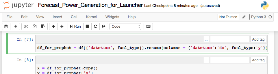
12. Save the notebook.
13. Stop and Commit the workspace session.
Create a wrapper file to execute.
1. Go back to the Files page.
2. Create a new file called forecast_launcher.sh.
3. Copy and paste the following code for the file and save it:
  papermill Forecast_Power_Generation_for_Launcher.ipynb forecast.ipynb -p start_date "$1" -p fuel_type $2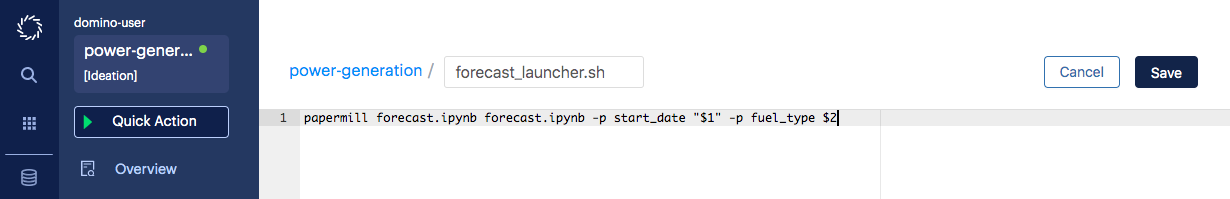
  The command breaks down as follows:
  
  papermill <input ipynb file> <output ipynb file> -p <parameter name> <parameter value>
  
  We will pass in our values as command line arguments to the shell script forecast_launcher.sh, which is why we have $1 and $2 as our parameter values.
Configure the Launcher.
1. Go to the Launcher page, found under the Publish menu in the sidebar.
2. Click New Launcher.
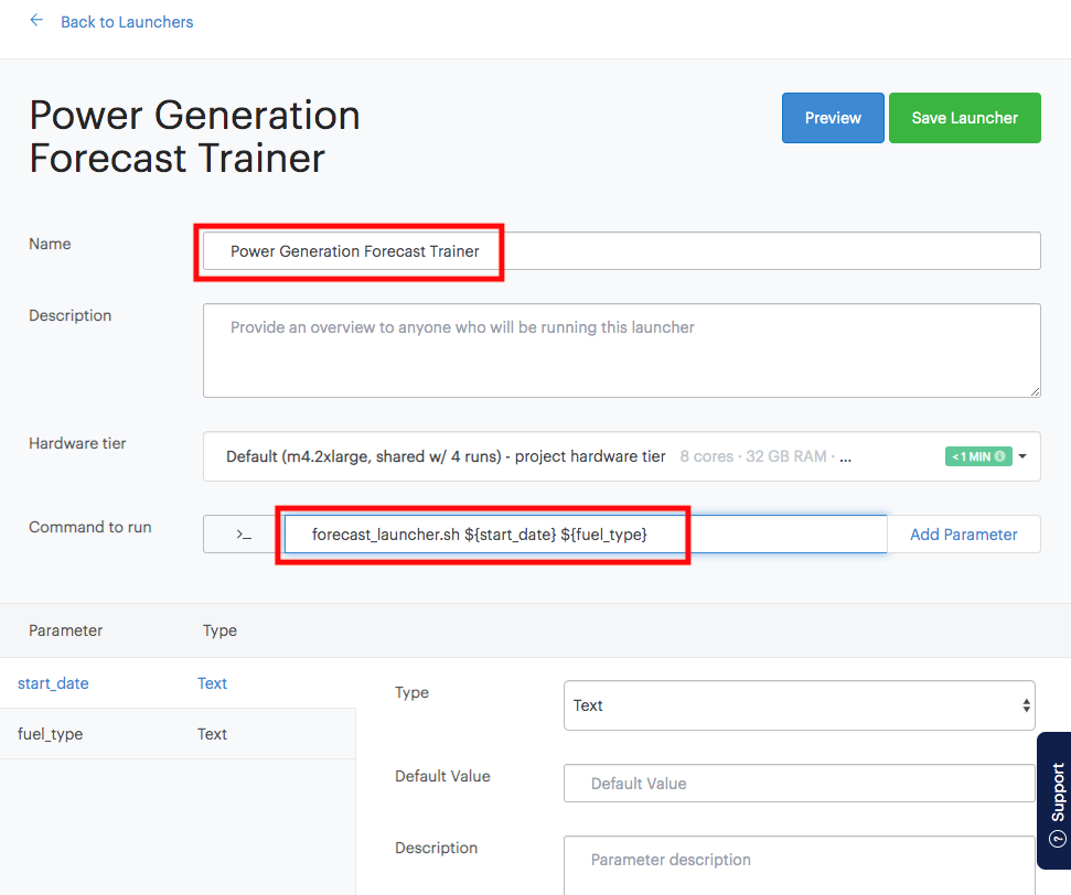
3. Name the launcher "Power Generation Forecast Trainer"
4. Copy and paste the following into the field "Command to run":
  forecast_launcher.sh ${start_date} ${fuel_type}
  You should see the following parameters:
5. Select the start_date parameter and change the type to Date.
6. Select the fuel_type parameter and change the type to Select (Drop-down menu).
7. Copy and paste the following into the Allowed Values field:
  CCGT, OIL, COAL, NUCLEAR, WIND, PS, NPSHYD, OCGT, OTHER, INTFR, INTIRL, INTNED, INTEW, BIOMASS, INTEM ,INTEL,INTIFA2,INTNSL
8. Click Save Launcher.
Try out the Launcher.
1. Go back to the main Launcher page.
2. Click Run for the "Power Generation Forecast Trainer" launcher.
3. Select a start date for the training data.
4. Select a fuel type from the dropdown.
5. Click Run

This will execute the parameterized notebook with the parameters that you selected. In this particular launcher, a new dataset was downloaded and the model was re-trained. Graphs in the resulting notebook represent the new dataset. You can see them in the Results tab.

When the run has been completed, an email will be sent to you and others that you optionally specified in the launcher with the resulting files. To learn how to customize the resulting email, see Set Custom Execution Notifications.

Model APIs

If you want your model to serve another application, you will want to serve it in the form of an API endpoint. Model APIs are scalable REST APIs that can create an endpoint from any function in a Python or R script. The Model APIs are commonly used when you need an API to query your model in near real-time.

For example, we created a model to forecast power generation of combined cycle gas turbines in the UK.

In this section, we will deploy an API that uses the model that we trained to predict the generated power given a date in the future. To do so, we will create a new compute environment to install necessary packages, create a new file with the function we want to expose as an API, and finally deploy the API.

Create a new compute environment.
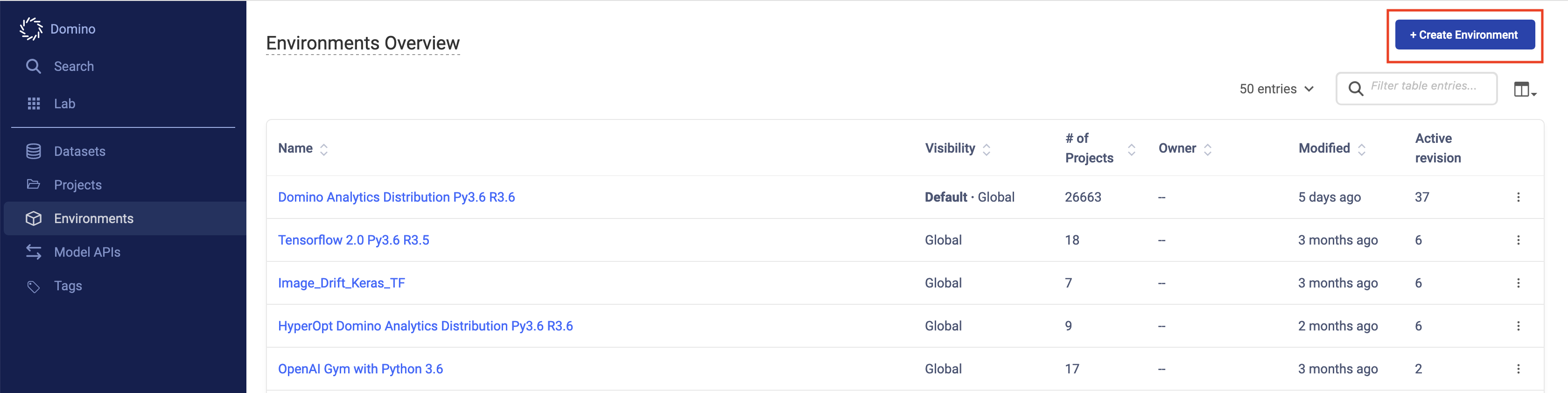
1. Go to the Environments page in Domino.
2. Click Create Environment.
3. Name the environment and enter a description for the new environment.
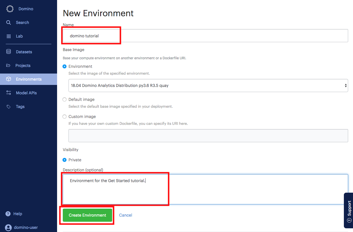
4. Click Create Environment.
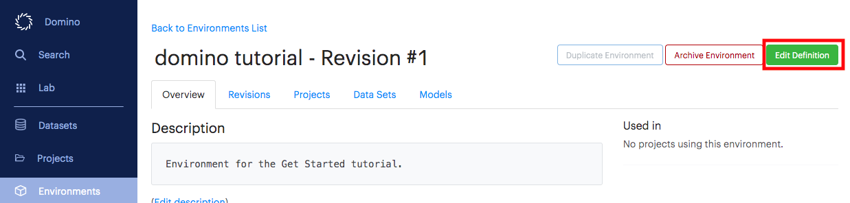
5. Click Edit Definition.
6. In the Dockerfile Instructions section, enter the following:
  RUN pip install "pystan==2.17.1.0" "plotly<4.0.0" "papermill<2.0.0" requests dash && pip install fbprophet==0.6
  RUN pip install "pystan==2.17.1.0" "plotly<4.0.0" "papermill<2.0.0" requests dash && pip install fbprophet==0.6
7. Scroll to the bottom of the page and click Build.
  
  This will start the creation of your new compute environment. These added packages will now be permanently installed into your environment and be ready whenever you start a job or workspace session with this environment selected. Note that PyStan needs 4 GB of RAM to install; reach out to your admin if you see errors so they can ensure that builds have the appropriate memory allocation.
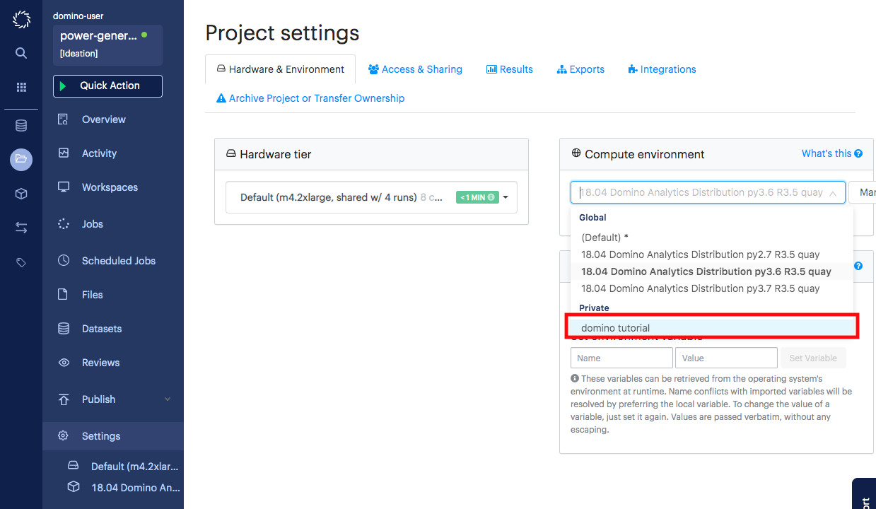
8. Navigate back to your project page and go to the Settings page.
9. Select your newly created environment from the Compute Environments dropdown menu.
Create a new file with the function we want to expose as an API
1. From the Files page of your project, click New File.
2. Name your file forecast_predictor.py.
3. Enter the following contents:
  import pickle import datetime import pandas as pd with open('model.pkl', 'rb') as f: m = pickle.load(f) def predict(year, month, day): ''' Input: year - integer month - integer day - integer Output: predicted generation in MW ''' ds = pd.DataFrame({'ds': [datetime.datetime(year,month,day)]}) return m.predict(ds)['yhat'].values[0]
  import pickle import datetime import pandas as pd with open('model.pkl', 'rb') as f: m = pickle.load(f) def predict(year, month, day): ''' Input: year - integer month - integer day - integer Output: predicted generation in MW ''' ds = pd.DataFrame({'ds': [datetime.datetime(year,month,day)]}) return m.predict(ds)['yhat'].values[0]
4. Click Save.
Deploy the API.
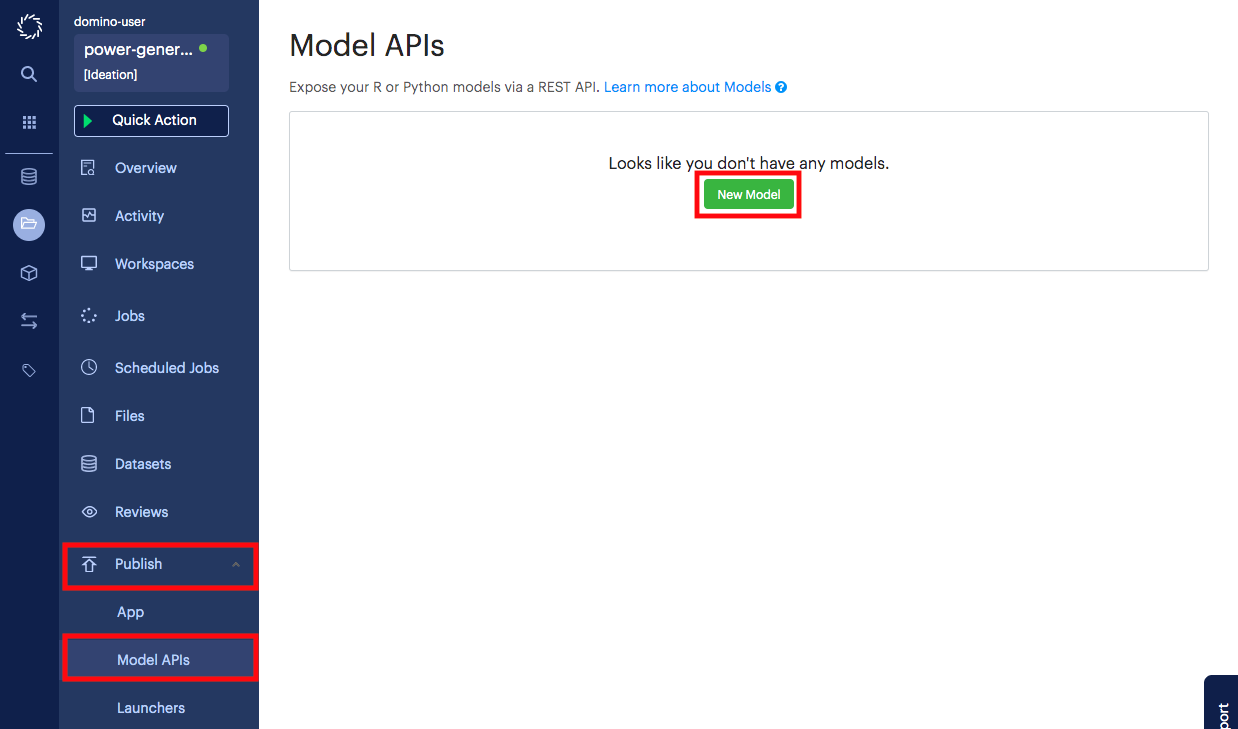
1. Go to the Publish/Model APIs page in your project.
2. Click New Model.
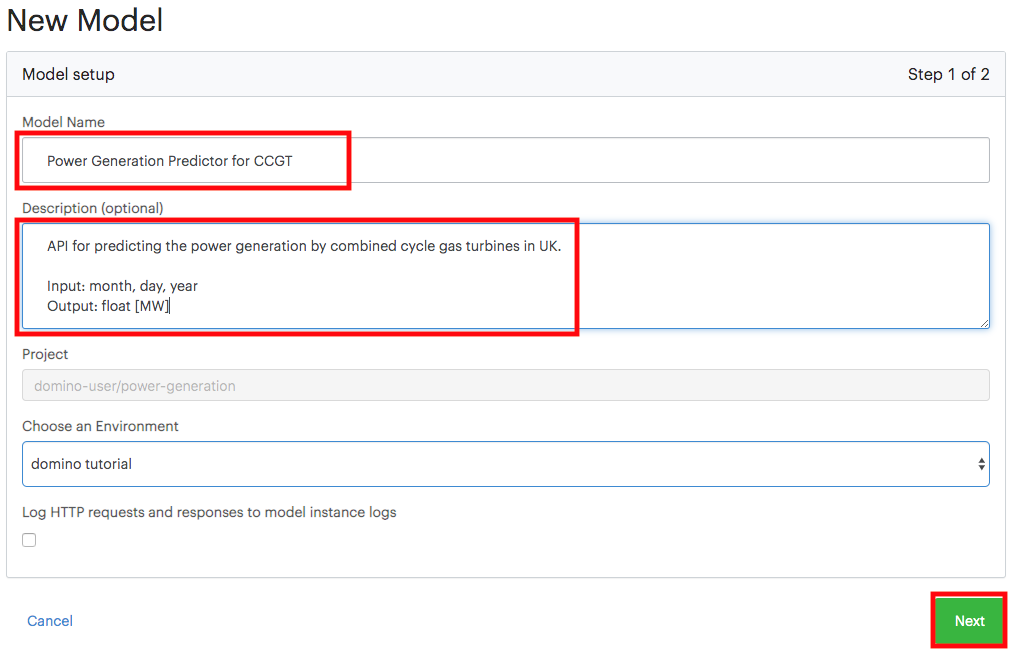
3. Name your model, provide a description, and click Next.
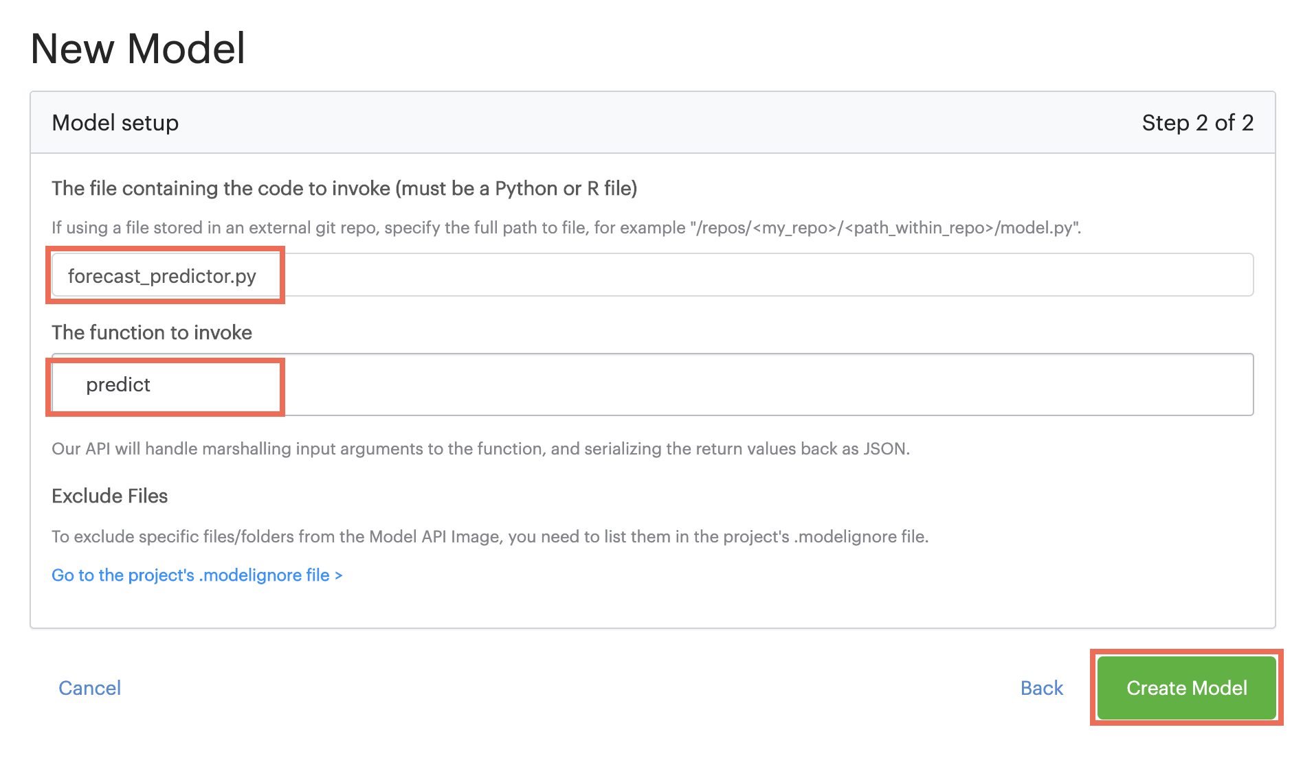
4. Enter the name of the file that you created in the previous step.
5. Enter the name of the function that you want to expose as an API.
6. Click Create Model.
Test the API.
1. Wait for the Model API status to turn to Running. This may take a few minutes.
2. Click the Overview tab.
3. Enter the following into the Request box in the tester:
  { "data": { "year": 2019, "month": 10, "day": 15 } }
  { "data": { "year": 2019, "month": 10, "day": 15 } }
4. Click Send. If successful, you will see the response in the pane.

As a REST API, any other common programming language will be able to call it. Code snippets from some popular languages are listed in the other tabs.

Model APIs are built as Docker images and deployed on Domino. You can export the model images to your external container registry and deploy them in any other hosting environment outside of Domino using your custom CI/CD pipeline. Domino supports REST APIs that enable you to programmatically build new model images on Domino and export them to your external container registry.

Web applications

When experiments in Domino yield results that you want to share with your colleagues, you can easily do so with a Domino App. Domino can host Apps built with many popular frameworks, including Flask, Shiny, and Dash.

While Apps can be significantly more sophisticated and provide far more functionality than a Launcher, they also require significantly more code and knowledge in at least one framework. In this section, we will convert some code that we developed when we trained a Python model and create a Dash app.

Add the app.py file, which will describe the app in Dash, to the project:

# -*- coding: utf-8 -*-
import dash
import dash_core_components as dcc
import dash_html_components as html
from datetime import datetime as dt
from dash.dependencies import Input, Output
import requests
import datetime
import os

import pandas as pd
import datetime
import matplotlib.pyplot as plt
from fbprophet import Prophet
import plotly.graph_objs as go

external_stylesheets = ['https://codepen.io/chriddyp/pen/bWLwgP.css']

app = dash.Dash(__name__, external_stylesheets=external_stylesheets)

app.config.update({'requests_pathname_prefix': '/{}/{}/r/notebookSession/{}/'.format(
    os.environ.get("DOMINO_PROJECT_OWNER"),
    os.environ.get("DOMINO_PROJECT_NAME"),
    os.environ.get("DOMINO_RUN_ID"))})

colors = {
    'background': '#111111',
    'text': '#7FDBFF'
}

# Plot configs
prediction_color = '#0072B2'
error_color = 'rgba(0, 114, 178, 0.2)'  # '#0072B2' with 0.2 opacity
actual_color = 'black'
cap_color = 'black'
trend_color = '#B23B00'
line_width = 2
marker_size = 4
uncertainty=True
plot_cap=True
trend=False
changepoints=False
changepoints_threshold=0.01
xlabel='ds'
ylabel='y'

app.layout = html.Div(style={'paddingLeft': '40px', 'paddingRight': '40px'}, children=[
    html.H1(children='Predictor for Power Generation in UK'),
    html.Div(children='''
        This is a web app developed in Dash and published in Domino.
        You can add more description here to describe the app.
    '''),
     html.Div([
        html.P('Select a Fuel Type:', className='fuel_type', id='fuel_type_paragraph'),
        dcc.Dropdown(
            options=[
                {'label': 'Combined Cycle Gas Turbine', 'value': 'CCGT'},
                {'label': 'Oil', 'value': 'OIL'},
                {'label': 'Coal', 'value': 'COAL'},
                {'label': 'Nuclear', 'value': 'NUCLEAR'},
                {'label': 'Wind', 'value': 'WIND'},
                {'label': 'Pumped Storage', 'value': 'PS'},
                {'label': 'Hydro (Non Pumped Storage', 'value': 'NPSHYD'},
                {'label': 'Open Cycle Gas Turbine', 'value': 'OCGT'},
                {'label': 'Other', 'value': 'OTHER'},
                {'label': 'France (IFA)', 'value': 'INTFR'},
                {'label': 'Northern Ireland (Moyle)', 'value': 'INTIRL'},
                {'label': 'Netherlands (BritNed)', 'value': 'INTNED'},
                {'label': 'Ireland (East-West)', 'value': 'INTEW'},
                {'label': 'Biomass', 'value': 'BIOMASS'},
                {'label': 'Belgium (Nemolink)', 'value': 'INTEM'},
            {'label': 'France (Eleclink)', 'value': 'INTEL'},
            {'label': 'France (IFA2)', 'value': 'INTIFA2'},
           {'label': 'Norway 2 (North Sea Link)', 'value': 'INTNSL'}
            ],
            value='CCGT',
            id='fuel_type',
            style = {'width':'auto', 'min-width': '300px'}
        )
    ], style={'marginTop': 25}),
    html.Div([
        html.Div('Training data will end today.'),
        html.Div('Select the starting date for the training data:'),
        dcc.DatePickerSingle(
            id='date-picker',
            date=dt(2020, 9, 10)
        )
    ], style={'marginTop': 25}),
    html.Div([
        dcc.Loading(
            id="loading",
            children=[dcc.Graph(id='prediction_graph',)],
            type="circle",
            ),
        ], style={'marginTop': 25})
])

@app.callback(
    # Output('loading', 'chhildren'),
    Output('prediction_graph', 'figure'),
    [Input('fuel_type', 'value'),
     Input('date-picker', 'date')])
def update_output(fuel_type, start_date):
    today = datetime.datetime.today().strftime('%Y-%m-%d')
    start_date_reformatted = start_date.split('T')[0]
    url = 'https://www.bmreports.com/bmrs/?q=ajax/filter_csv_download/FUELHH/csv/FromDate%3D{start_date}%26ToDate%3D{today}/&filename=GenerationbyFuelType_20191002_1657'.format(start_date = start_date_reformatted, today = today)
    r = requests.get(url, allow_redirects=True)
    open('data.csv', 'wb').write(r.content)
    df = pd.read_csv('data.csv', skiprows=1, skipfooter=1, header=None, engine='python')
    df.columns = ['HDF', 'date', 'half_hour_increment',
                'CCGT', 'OIL', 'COAL', 'NUCLEAR',
                'WIND', 'PS', 'NPSHYD', 'OCGT',
                'OTHER', 'INTFR', 'INTIRL', 'INTNED', 'INTEW', 'BIOMASS', 'INTEM',
                'INTEL','INTIFA2', 'INTNSL']
    df['datetime'] = pd.to_datetime(df['date'], format="%Y%m%d")
    df['datetime'] = df.apply(lambda x:
                          x['datetime']+ datetime.timedelta(
                              minutes=30*(int(x['half_hour_increment'])-1))
                          , axis = 1)
    df_for_prophet = df[['datetime', fuel_type]].rename(columns = {'datetime':'ds', fuel_type:'y'})
    m = Prophet()
    m.fit(df_for_prophet)
    future = m.make_future_dataframe(periods=72, freq='H')
    fcst = m.predict(future)
    # from https://github.com/facebook/prophet/blob/master/python/fbprophet/plot.py
    data = []
    # Add actual
    data.append(go.Scatter(
        name='Actual',
        x=m.history['ds'],
        y=m.history['y'],
        marker=dict(color=actual_color, size=marker_size),
        mode='markers'
    ))
    # Add lower bound
    if uncertainty and m.uncertainty_samples:
        data.append(go.Scatter(
            x=fcst['ds'],
            y=fcst['yhat_lower'],
            mode='lines',
            line=dict(width=0),
            hoverinfo='skip'
        ))
    # Add prediction
    data.append(go.Scatter(
        name='Predicted',
        x=fcst['ds'],
        y=fcst['yhat'],
        mode='lines',
        line=dict(color=prediction_color, width=line_width),
        fillcolor=error_color,
        fill='tonexty' if uncertainty and m.uncertainty_samples else 'none'
    ))
    # Add upper bound
    if uncertainty and m.uncertainty_samples:
        data.append(go.Scatter(
            x=fcst['ds'],
            y=fcst['yhat_upper'],
            mode='lines',
            line=dict(width=0),
            fillcolor=error_color,
            fill='tonexty',
            hoverinfo='skip'
        ))
    # Add caps
    if 'cap' in fcst and plot_cap:
        data.append(go.Scatter(
            name='Cap',
            x=fcst['ds'],
            y=fcst['cap'],
            mode='lines',
            line=dict(color=cap_color, dash='dash', width=line_width),
        ))
    if m.logistic_floor and 'floor' in fcst and plot_cap:
        data.append(go.Scatter(
            name='Floor',
            x=fcst['ds'],
            y=fcst['floor'],
            mode='lines',
            line=dict(color=cap_color, dash='dash', width=line_width),
        ))
    # Add trend
    if trend:
        data.append(go.Scatter(
            name='Trend',
            x=fcst['ds'],
            y=fcst['trend'],
            mode='lines',
            line=dict(color=trend_color, width=line_width),
        ))
    # Add changepoints
    if changepoints:
        signif_changepoints = m.changepoints[
            np.abs(np.nanmean(m.params['delta'], axis=0)) >= changepoints_threshold
        ]
        data.append(go.Scatter(
            x=signif_changepoints,
            y=fcst.loc[fcst['ds'].isin(signif_changepoints), 'trend'],
            marker=dict(size=50, symbol='line-ns-open', color=trend_color,
                        line=dict(width=line_width)),
            mode='markers',
            hoverinfo='skip'
        ))

    layout = dict(
        showlegend=False,
        yaxis=dict(
            title=ylabel
        ),
        xaxis=dict(
            title=xlabel,
            type='date',
            rangeselector=dict(
                buttons=list([
                    dict(count=7,
                         label='1w',
                         step='day',
                         stepmode='backward'),
                    dict(count=1,
                         label='1m',
                         step='month',
                         stepmode='backward'),
                    dict(count=6,
                         label='6m',
                         step='month',
                         stepmode='backward'),
                    dict(count=1,
                         label='1y',
                         step='year',
                         stepmode='backward'),
                    dict(step='all')
                ])
            ),
            rangeslider=dict(
                visible=True
            ),
        ),
    )
    return {
        'data': data,
        'layout': layout
    }

if __name__ == '__main__':
    app.run_server(port=8888, host='0.0.0.0', debug=True)

Add an app.sh file to the project, which provides the commands to instantiate the app:
```
python app.py
```
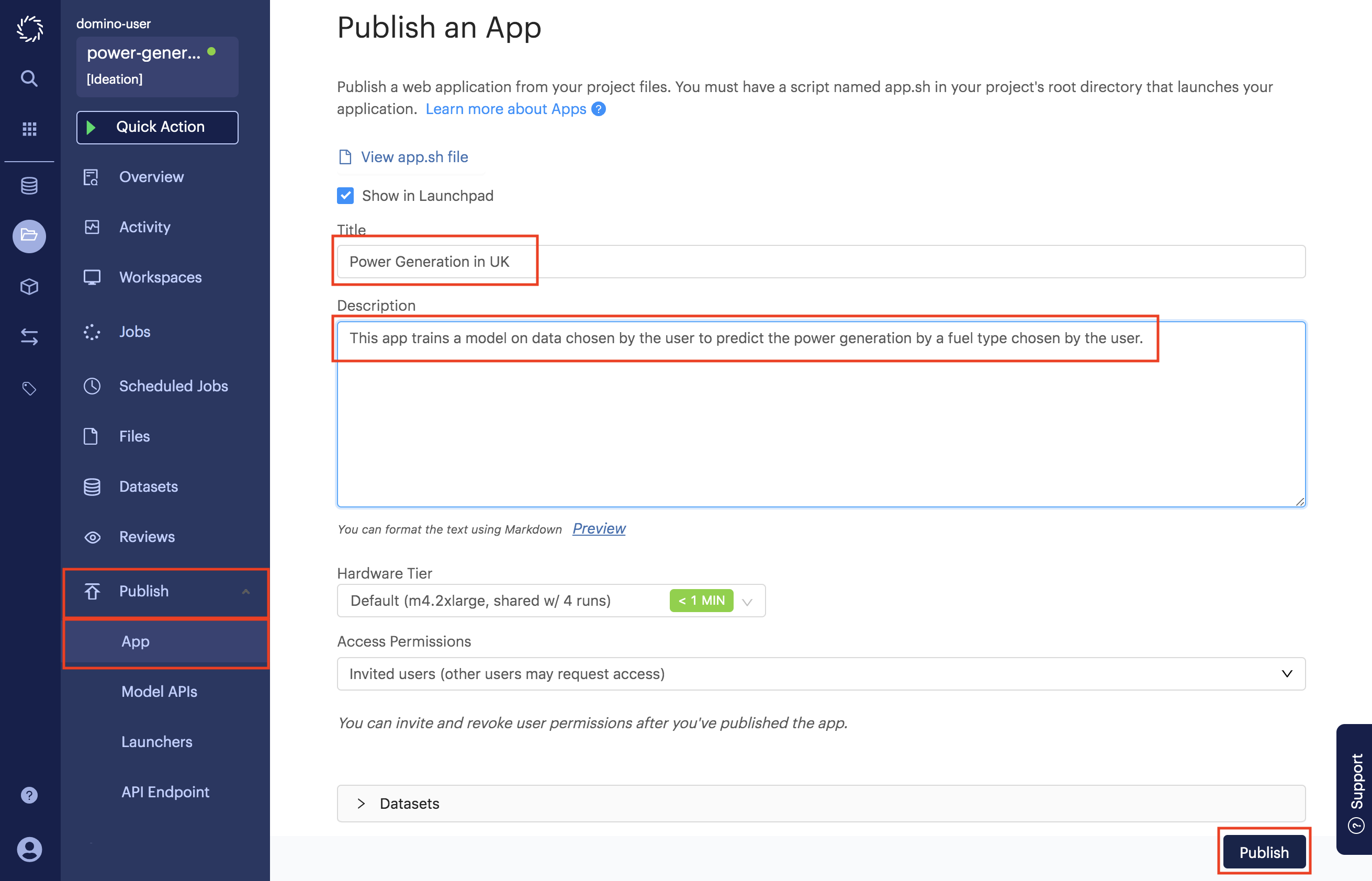
Publish the App.
1. Go to the App page under the Publish menu of your project.
2. Enter a title and a description for your app.
3. Click Publish.
4. After the app status appears as Running (which might take a few minutes), you can click View App to open it.
Share your app with your colleagues.
1. Go to the Publish/App page and select the Permissions tab.
2. Invite your colleagues by username or email.
3. Or, toggle the Access Permissions level to make it publicly available.

See Domino Apps for more information.

User Guide

Admin Guide