Use the Scheduled Jobs feature in Domino to run a script regularly.
You can create reports in MATLAB using the publish() function and the
robust MATLAB
Report Generator. To simplify things, in this tutorial, you will use
the publish() function, which uses a MATLAB m file as a document
template.
Imagine that you receive data daily about Berlin’s weather. You want to generate a scheduled email visualizing this data, as well as the forecasted number of hot days in the next 365 days.
To do that, create the following files:
-
An
m.file, based on your Live Script, that will:-
Load Berlin weather data from a URL.
-
Prepare the data.
-
Generate predictions using the model you create with the data.
-
Call the
publish()function.
-
-
An
m.file that will be your report template that shows:-
A weather prediction plot.
-
The number of predicted hot days.
-
-
Go to Workspaces and click Open Last Workspace.
-
Go to New > Script to create a new file.
-
Click Save > Save As to name it
predictWeatherReport.m. -
Copy and paste the following code to your file. This code initializes a
structto hold the results, defines a hot day temperature threshold (in degrees Celsius), downloads the current data for Berlin weather, and saves it to the workspace. It will read the downloaded file into a table format.%% Initial setup result = struct; hotDayThreshold = 30; %% Download data file urlString = "https://www.ncei.noaa.gov/data/global-historical-climatology-network-daily/access/GME00121150.csv"; if ~isfolder("data") mkdir('data'); end savedFileName = sprintf("%s%s%s", "data", filesep, "berlin.csv"); websave(savedFileName, urlString); %% Read the downloaded file opts = detectImportOptions(savedFileName); opts.SelectedVariableNames = {'DATE', 'PRCP', 'TMIN', 'TMAX'}; opts = setvartype(opts, {'DATE','PRCP','TMIN','TMAX'},{'datetime','double', 'double', 'double'}); stationWeatherTbl = readtable(savedFileName, opts); -
To prepare the data, copy and paste the following code that will start with data from the year 1999, adjust the temperature data to full degrees, and complete missing data. If there are less than 1000 rows of data, the data will stop processing.
%% [stationWeatherTbl.year, stationWeatherTbl.month, stationWeatherTbl.day] = ymd(stationWeatherTbl.DATE); % MATLAB strength stationWeatherTbl = stationWeatherTbl(stationWeatherTbl.year > 1999 & stationWeatherTbl.year < max(stationWeatherTbl.year), :); stationWeatherTbl.TMAX = stationWeatherTbl.TMAX/10; stationWeatherTbl.TMIN = stationWeatherTbl.TMIN/10; stationWeatherTbl = fillmissing(stationWeatherTbl, 'linear'); %% check if there is enough data for prediction dataRows = size(stationWeatherTbl, 1); if dataRows < 1000 disp('Not enough data for prediction'); result.error = 'Not enough data for prediction'; return; end -
Copy and paste the following code which will load the model that you created previously and save it into a
.matfile. Then, it will create the table to use as input with the updated data that was read from the URL previously.%% Check if we have a model for this weather station modelFileName = sprintf("%s%s%s%s", "models", filesep, "weatherStationId", ".mat"); % make sure we have a folder for the models if ~isfolder('models') mkdir('models') end if ~isfile(modelFileName) disp('Training model for weather station...') cv = cvpartition(stationWeatherTbl.year, 'Holdout', 0.3); dataTrain = stationWeatherTbl(cv.training, :); [weatherModel, validationRMSE] = trainRegressionModel(dataTrain); % display prediction precision doneMessage = sprintf('%s%d', "Done. Model RMSE:", validationRMSE); disp(doneMessage); save(modelFileName, 'weatherModel'); else load(modelFileName, 'weatherModel'); end%% Create table for future date prediction todayDate = datetime('today'); daysIntoFuture = 365; endDate = todayDate + days(daysIntoFuture); predictedMaxTemps = table('Size', [daysIntoFuture+1 7], 'VariableTypes', {'datetime', 'double', 'double', 'double', 'double', 'double', 'double'}, 'VariableNames', stationWeatherTbl.Properties.VariableNames); x=1; for i=todayDate:endDate % get the average perception and minimum temps on this date [y, m, d] = ymd(i); minTemps = stationWeatherTbl.TMIN(stationWeatherTbl.month == m & stationWeatherTbl.day == d); prcps = stationWeatherTbl.PRCP(stationWeatherTbl.month == m & stationWeatherTbl.day == d); curMinTemp = NaN; [historicalRowCount z] = size(minTemps); randomRow = randi([1 historicalRowCount]); curMinTemp = minTemps(randomRow); predictedMaxTemps.TMIN(x) = curMinTemp; randomRow = randi([1 historicalRowCount]); predictedMaxTemps.PRCP(x) = prcps(randomRow); predictedMaxTemps.DATE(x) = i; predictedMaxTemps.year(x) = y; predictedMaxTemps.month(x) = m; predictedMaxTemps.day(x) = d; predictedMaxTemps.TMAX(x) = 0; x = x+1; end -
Copy and paste the following code that will run the model and load the
resultstruct with the prediction.%% yFit = weatherModel.predictFcn(predictedMaxTemps); predResult = table(predictedMaxTemps.DATE, yFit, 'VariableNames', {'Date', 'Predicted TMAX'}); result.predictedTemps = predResult; hotWeatherDaysIdx = predResult(predResult.("Predicted TMAX") > hotDayThreshold, :); result.hotDayCountPrediction = height(hotWeatherDaysIdx); -
Copy and paste the following code to share the prediction result with the template in the
.mstfile. You must include this because thepublish()function runs in isolation from the workspace. To ensure the data file has a unique name for each run of this script, this code uses the Domino environment variable for the run number.%% save data to file dominoRunId = getenv('DOMINO_RUN_NUMBER'); outputFileName = sprintf('%s%s%s', 'results', filesep, 'predictData_', string(dominoRunId)); save(outputFileName, 'result'); -
Copy and paste the following code to call the
publish()function. The report will be published to a subfolder of theresults/folder, along with the number of the current run in the filename.%% Publish the report % options for the report pub_options.format = 'pdf'; % hide the report code pub_options.showCode = false; pub_options.outputDir = sprintf('%s%s%s', 'results', filesep, dominoRunId); doc = publish('predictWeatherReportTemplate.m', pub_options); -
Click Save.
-
To create the report template, create a script named
predictWeatherReportTemplate.m. Copy and paste the following code to load the data. This tutorial uses the following format for the filename when loading the data:results/predictData_<Domino Run Number>. The data is stored in a variable calledresult.dominoRunId = getenv('DOMINO_RUN_NUMBER'); inputFileName = sprintf('%s%s%s', 'results', filesep, 'predictData_', string(dominoRunId)); load(inputFileName, 'result'); -
Copy and paste the following code to add a title to the template. In this MATLAB template, comments will be rendered as markup. For more information, see MATLAB’s documentation about markup comments for publishing.
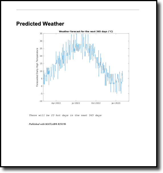
%% Predicted Weather -
Copy and paste the following to add the plot with the data that you loaded previously and show the hot day predictions as output.
predResult = result.predictedTemps; plot(predResult.Date, predResult.("Predicted TMAX")); titleText = "Weather forecast for the next 365 days (\circC)"; title(titleText); ylabel ('Forecasted Daily High Temperature') %% countPredictionText = sprintf("%s%d%s", "There will be ", ... result.hotDayCountPrediction, " hot days in the next 365 days"); disp(countPredictionText); -
Click Save.
-
Click File Changes in the navigation bar. Then, click Sync All Changes to save and commit your changes.
-
To test the
predictWeatherReport.mfile, type the following in the Command Window to call the file and press Enter:predictWeatherReportThe following graph shows the weather forecast:
A new folder and new file are created in the
results/folder.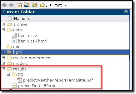
-
Save and sync your changes.
-
Stop your MATLAB session. Click the Domino icon and then, in the navigation pane, click Jobs > Schedules.
-
Click Schedule a Job.
-
Type a name for the job and type
predictWeatherReport.mas the file to run for this job. -
Select a hardware tier.
-
Confirm that your environment is the same as the one in which you developed your model.
-
Click Next.
-
-
On the Attach Compute Cluster page, select none and click Next
-
Schedule the job to run every weekday. Leave the Run sequentially option checked. Click Next.
-
Type the email addresses for those to notify when the job is complete. Click Create.
You have scheduled a job that will use your MATLAB code to generate a report. You can also go to the Jobs page to run the job on an ad-hoc basis.
To learn how to customize the resulting email, see Set Custom Execution Notifications.